After all the fun building up the spectrogram dataset in the last post, it’s now time to see how they’ll be handled by some of the fancy computer vision models that everyone loves to use these days! I decided to go with the ResNet family of models since it’s what I’ve been playing with in the fastai course and getting good performance, so I stuck with this choice to make it simple *

I started by loading my images and splitting 20% of them off into a validation set **, with no additional data augmentation. The sliding window approach with overlaps that I described in the previous post to split longer sounds into spectrograms representing exactly 10 seconds of sound should already act as some data augmentation. Also, I don’t want the images distorted/altered in any way because xy positions and colour are all on a fixed scale across all images!

The first model that I tried training was using pretrained weights of the resnet18 architecture. I decided to use a pretrained model because there should be useful edge/colour detection features that would transfer to the data contained in the spectrograms, even though the original model was trained to classify photographs of real objects. Apart from training for 10 epochs, everything else went with the standard Learner.fine_tune options from fastai.

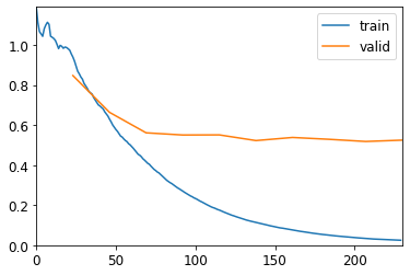
As you can see from the plot of the training and validation losses above, training seemed to go pretty smoothly, with the validation loss leveling off fairly quickly the training loss dropping for a bit longer. The x-axis doesn’t go from 1-10 epochs because it shows the loss per batch of images sent to the GPU during training, so each epoch was about 22 batches in that scale. The error rate on the validation set isn’t on the plot, but it was about 14% by the end of training. That’s not bad for my very first go at forcing a vision model that was trained on real photographs classify images representing sounds!

But let’s see how much further we can get with some changes in training or architecture. The easiest setting to try changing is the initial learning rate during training. Fastai’s fine_tune method does vary the learning rate as it goes along, but the default initial value is 0.001 and I know that the best learning rate is a hyperparameter that can vary a lot between models and datasets. Luckily, I don’t have to try a lot of different learning rates and compare them manually, because fastai has a handy Learner.lr_find method that automaticaly tests a lot of different learning rates on a small sample of the dataset, plots the loss on a graph and tells you two choices that should be safe.

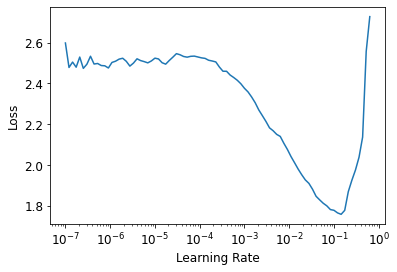
The plot looks nicely behaved, with the loss exploding as the rate approaches 1, a flattish region towards lower values and then a nice slope down to a minimum value around 0.1. I picked the first recommended value (0.014), which is 1/10 of the learning rate of the minimum point, because the other option (highest slope) was too close to the 0.001 default and probably wouldn’t change much. Training with this learning rate did produce some noticeable improvements, with the validation loss leveling off only after batch 100 or so, at a lower value than in the first training run. This was also reflected in the validation set error rate that was around 7.4%!

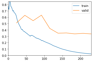
Since this was a pretrained models for classification of real photos, I wondered whether everything it had to learn about cats, dogs, cars, humans, and all the other random things in its original training set could be hindering its performance on the very simple plots I was feeding it! So I started with a copy of the network with random weights, picked the optimal learning rate as before and let it run free for 50 epochs:

As you can see the validation loss was a lot more spiky this time and took much longer to stabilise! The error rate reached a minimum of just over 8% around epoch 30, but then gradually rose back to about 10% at the end of training. That got pretty close to the best performance I got from the pretrained model, but never managed to beat it.

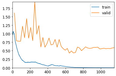
Another hyperparameter I tested was a deeper architecture (ie, more layers) for the network. I did the same three training runs as I decribed for the resnet18 architecture above, but using the resnet34 architecture, which performs better on real photos. I won’t repeat the plots because they look very similar, but for the training runs with default settings and also the longer one starting from random weights, I got slightly worse performance than I saw on resnet18. However, for the run starting from the pretrained model and using the learning rate finder, the final validation error rate was 6%!

It really does seem like the best way to produce a classifier for these bird sounds as spectrograms was with picking an appropriate learning rate for the pre-trained models, out of the set of options I tested here. Since the error rates of the two best options were still very close (6% and 7.4%) and I also wanted to see how the other models would perform on a held out set of data, I ran predictions on the entire test set for all 6 models.

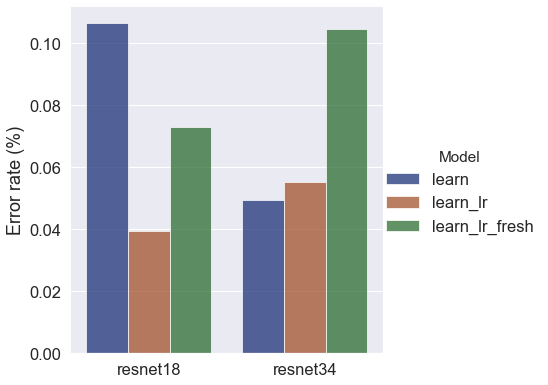
Against the test set, the resnet18 pretrained model with the optimal learning rate (resnet18_lr) and the deeper architecture with the both learninr rates (resnet34 and resnet34_lr) were clearly the best performers. The “fresh” models (with randomly-initialised weights) both performed distinctly worse, along with the default learning rate resnet18.

From the loss values during training I was starting to think that the deeper architecture was more prone to overfitting, which was leading to the higher error rates on the validation set. But the pattern didn’t hold on the test set, so this variability may be pointing towards a need for more optimisation/tweaking of training conditions. I may revisit this in yet another post in this series, once I’ve done a bit more reading and exploration of what’s going on during model training.

For now, let’s just have a look at how the best model was performing (resnet18_lr):

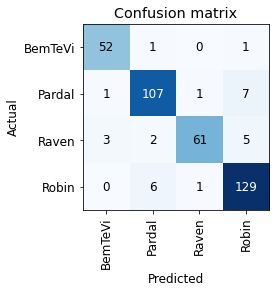
There’s no class in the confusion matrix that looks obviously troublesome and there were mispredictions for all classes. There were just two false positive BemTeVi predictions and two false negative Raven predictions, with all others having >=4 errors of each type. Let’s have a glance over at the images with the highest losses, which made the model “more confused”:

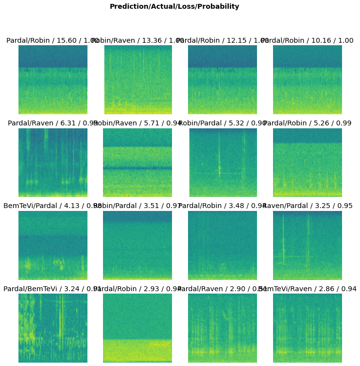
The first things that jumped out at me from looking at that array was that all images along the top row and all the images down the second vertical column from the left were a bit featureless, with not many of the clearly-visible vertical lines and squiggles that I’ve learned (and I hope the models did as well!) to spot in the spectrograms. I didn’t inspect all the 2k+ images manually, so there might be quite a few in the dataset that have long quiet stretches or enough background noise to drown out the actual sounds made by the birds.

There are a few others that do have more visible features, including some with a lot of squiggles packed very closely together (4th row from top, 1st column from left is a good example). I haven’t listened to many of the actual recordings, but this latter case could actually have vocalisations from both the mispredicted Pardal/Sparrow and the labeled BemTeVi/Kiskadee, given that these birds co-occur at least in Brazil and possibly other places. I believe this is a weakness of how data is labeled in the iNaturalist database, since users deposit recordings as “observations” for specific animal species but birds are not very polite and don’t always stay quiet while the human birdwatcher is recording their neighbours that belong to other species!

As I was writing the post, I also went back to check some aspects of the previous one and spotted a potential problem in my train-validate-test split: my overlapping sliding window approach to producing the spectrogram images may be leaking some data between sets. Looking at the last image from the last post will hopefully make this point clear.

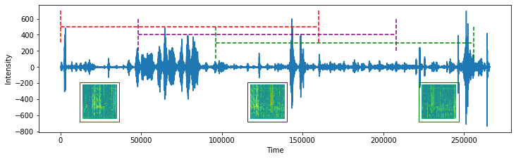
Since I split the images randomly into the three sets, there may be bits of data present in more than one set, which means that models may be seeing parts of the validation or test sets during training. Using the recording depicted above as an example, let’s assume the spectrogram highlighted in red went to the test set, then the purple one went to validation and the green one to test. In that case, the part of the red bar that overlaps the green and purple bars represents some leakage of the validation and test data into the training set, which could mean I’m overestimating model performance in the metrics I extracted at the end of the process. I could go back and generate a new dataset with the train-validate-test splits taking place before making the spectrograms with the sliding window, so I’ll keep this in mind for future work with this data.

Even though the focus of this post was on model training and I did get some promising results, I think these last conclusions are telling me that I’d get more improvements from further work on the dataset itself than if I just kept hacking at models and hyperparameters! And, as I said above, I may revisit the dataset and these models in a future post. For now though, my plan is to first package the best model as is into a very simple web app that will let anyone upload a .wav file with the vocalisation of either a sparrow, a kiskadee, a raven or a robin and receive an answer from this classifier.

Footnotes

* I did just find a nice and detailed blog post explaining the architecture of the ResNet models, which I’ll read once I’m done with this post and might also be useful to anyone who’s curious.

** You might remember that I already split 20% of all the spectrograms into a test set, which I’ll only touch towards the end of this post, when I compare models trained with different sets of hyperparameters.